Magnetic Field Re-configuration Associated With a Slow Rise Eruptive X1.2 Flare in NOAA Active Region 11944

1 Introduction

Coronal Mass Ejections (CMEs) have long been identified as a prime cause of large, non-recurrent geomagnetic storms (e.g., Burlaga et al., 1981; Tsurutani et al., 1988; Gosling et al., 1990; Zhang et al., 2007). Solar plasma and magnetic fields ejected into the heliosphere as a result of an eruption are further propelled into interplanetary space where they may encounter the Earth’s magnetosphere and produce large southward excursions of the interplanetary magnetic field. Interplanetary CMEs observed near the Earth often exhibit a flux rope structure (e.g., Burlaga et al., 1981; Marubashi et al., 2015), meaning that they harbor a large-scale, coherent loop-like structure with a large amount of twist. Many studies have illustrated that the sense of the magnetic twist and the direction of the fields in ICMEs matches those of the source region, thus opening a pathway for predicting the likelihood of geomagnetic storms (e.g., Pevtsov & Canfield, 2001; Yurchyshyn et al., 2005; Gopalswamy et al., 2007; Marubashi et al., 2015, and references therein) and the CME speed may be related to the magnitude of the associated storm (e.g., Srivastava & Venkatakrishnan, 2004; Yurchyshyn et al., 2004; Yurchyshyn et al., 2005).

CMEs most frequently erupt from solar active regions (ARs) and are often accompanied by solar flares (Zhang et al., 2007). During an eruption event, stored free energy is released from complex magnetic structures of an AR through series of magnetic reconnections. While current CME models commonly assume the presence of a magnetic flux rope (MFR) in the ejecta, they differ in the way the initiation of the eruption is treated. In some models, an MFR is required to exist prior to the eruption (e.g., Chen & Shibata, 2000; Fan & Gibson, 2004; Török & Kliem, 2005; Kliem & Török, 2006), while in other models the eruption begins from reconnection in a sheared magnetic arcade (SMA) and an unstable MFR is formed in the process of the event (Antiochos et al., 1999; Moore et al., 2001; Karpen et al., 2012). Meanwhile, some studies also discussed borderline cases, when the detailed topological analysis reveals weakly twisted MFRs, and field line plots show the presence of an SMA (Aulanier et al., 2009; Savcheva et al., 2012). More details on pre-eruptive magnetic configurations may be found in a recent comprehensive review by Patsourakos et al. (2020). Real life eruptions may not follow any particular eruption model and studies of pre-eruptive magnetic fields are vital for understanding and predicting solar eruptions.

Solar ARs present various magnetic structures and topologies and some of them are prone to eruption (e.g., Kusano et al., 2012; Toriumi et al., 2017). One of the global goals of solar physics is to understand how an AR evolves toward eruption. From a practical point of view, we would like to know where and when the next eruption will occur. Most of the modern forecasting research (e.g., Falconer et al., 2014; Barnes et al., 2016; Leka et al., 2019a,b) is based on analysis of observed photospheric magnetograms provided by Helioseismic and Magnetic Imager (HMI) instrument (Scherrer et al., 2012; Schou et al., 2012) on board Solar Dynamics Observatory (SDO, Pesnell et al., 2012). However, photospheric measurements alone do not uniquely represent the complexity of coronal magnetic fields rooted in the photosphere, which is of vital importance for understanding the eruption process. Energy needed to expel twisted magnetic structures and plasma in the interplanetary space is stored in the corona above an AR is thought to be generated by plasma flows in the photosphere and the convection zone. Moreover, structural organization of the coronal fields is also responsible for the initiation of eruption, since their continuous evolution may lead to an unstable state, when the force balance is disrupted and a MFR or a SMA may erupt.

Several studies took advantage of the advances in modeling of AR coronal fields and used modeling results to address flare forecasting by analyzing, for example, pre-flare magnetic energy balance (e.g., Gupta et al., 2021), the rate of decay of coronal fields (e.g., Jing et al., 2018), and determining the pre-eruptive configuration (e.g., Duan et al., 2019; Kusano et al., 2020). A recent comprehensive comparison of flare forecasting methods is given in Park et al. (2020).

Here we use series of non-linear force-free field (NLFFF) extrapolations to explore evolution of an AR configuration toward an eruptive state. We analyze the model configurations using twist and q-factor maps (Titov et al., 2002; Titov, 2007; Liu et al., 2016) and their complexity is measured by using a cancellation exponent (e.g., Ott et al., 1992; Yurchyshyn et al., 2000a) and the decay index (Kliem & Török, 2006).

2 Data and Methods

We use HMI magnetic field measurements as a boundary condition to perform the magnetic field extrapolation. HMI observes the full solar disk in the Fe I 617.3 nm absorption line with a spatial resolution of 1^″. To generate the photospheric level vector magnetic field boundary conditions, we used HMI data rebinned to 1 Mm pixel scale transformed to a local Cartesian coordinate system using the same Cylindrical Equal Area (CEA) projection (Thompson, 2006) used to produce the standard hmi.sharp_cea_720s series data (SHARP, Bobra et al., 2014). Our customized coordinate transformations use a reference point exactly centered on the base of the Cartesian box to ensure that when the model is placed in the proper 3D orientation relative to the observer, the base maps are projected onto their line-of-sight (LOS) counterparts with minimum distortion.

Atmospheric Imaging Assembly (AIA, Lemen et al., 2012) provides full-disk images of the solar corona in a broad UV range nearly simultaneously with an image scale of 0^″.6 per pixel and a cadence of 12 s covering a wide and nearly continuous coronal temperature range of 0.7–20 MK. AIA 17.1 and 160 nm images were used to determine timing and location of initial flare brightenings as well as to verify the coronal field extrapolation results.

2.1 Coronal Field Extrapolation

Coronal field extrapolation was performed using Fleishman et al. (2017) tool that exploits the optimization method developed by Wheatland et al. (2000). An optimization method allows us to transform an initial magnetic configuration to a final NLFFF configuration. Fleishman et al. (2017) method follows an approach of using the weight function presented in Wiegelmann (2004). Authors modified the original method so that no pre-processing of the photospheric boundary conditions is performed and the initial approximation for the magnetic field for the most sparse grid is the potential field, while for each next, denser grid, the initial field is taken as an appropriate interpolation of the final (NLFFF) state of the previous grid. The numerical realization of this approach is part of the GX Simulator package (Nita et al., 2015, 2018), which is freely available from the SolarSoft IDL library.

2.2 Magnetic Flux Rope Identification Approach

Coronal field extrapolations allow us to search for possible signatures of a MFR using the squashing factor, Q, and magnetic twist, T_W, parameters calculated inside the extrapolated volume (Titov et al., 2002; Titov, 2007; Liu et al., 2016). The definitions of an MFR found in literature are not very strict and often magnetic twist (Berger & Prior, 2006) is used as a discriminator to identify a MFR. This parameter defines the number of turns that two close field lines make around each other and it is often accepted that a MFR is an ensemble of field lines with a twist exceeding unity. Here we adopt the definition of a MFR presented in Patsourakos et al. (2020). A MFRs is a twisted structure with a magnetic axis that follows a PIL, a current channel, and twist extending over the full length of the magnetic axis. MFRs are not expected to exhibit uniform twist along the entire length. It was also suggested that when a MFR is twisted in excess of a critical value T_Wc > 1.25, kink instability may develop leading to a subsequent eruption (e.g., Hood & Priest, 1981; Baty, 2001; Fan & Gibson, 2003; Török & Kliem, 2003). Generally speaking, MFRs are associated with the presence of extended, often lane-shaped high Q-structures located near a polarity inversion line (PIL) (Liu et al., 2016). Hereinafter we will refer to them as high Q-lanes. It should be noted however, that not every strong Q-lane indicates the presence of a MFR, since short Q lane also may appear in connection with SMAs. Strong Q-lanes may be viewed as the photospheric footprint of quasi-separatix layers (QSL) which are the interface between two magnetic flux systems. They are known to display a strong connectivity gradient (Titov et al., 2002; Titov, 2007; Liu et al., 2016).

3 Results

In Figure 1 we show an HMI magnetogram (top left), AIA 17.1 (top right) and 160 nm (bottom right) images, and results of the coronal field extrapolation plotted over the HMI magnetogram. Contours in the AIA 160 nm panel outline initial brightenings associated with an X1.2 flare that erupted on 2014 January 7 at 18:04 UT, peaked at 18:32 UT and ended at 18:58 UT. This was a slow rise flare followed by a fast CME and a coronal wave. We note that the first short lived and compact brightenings (flare precursors) appeared at the site of eruption about 20 min prior to the flare onset indicating on possible pre-flare activity at this location. This event was at the focus of two case (Wang et al., 2015; Zheng et al., 2016) and several statistical (Falconer et al., 2016; Toriumi et al., 2017; Toriumi & Takasao, 2017; Lu et al., 2019; Duan et al., 2019, 2021) studies. The flare erupted at the outskirt of the AR, south-west of the leading sunspot and away from the major PIL. Zheng et al. (2016) noted a complex structure of flare ribbons located on both sides of a chromospheric filament. One of the ribbons was visible for about 3 h after the flare onset and it is worth noting that the Hα filament was visible at that moment as well¹.

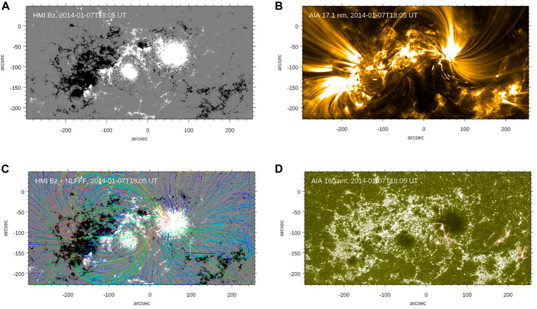
FIGURE 1. NOAA AR 11944 as it appeared in an HMI magnetogram (A) as well as AIA 17.1 and 160 nm imaging data (B,D) on 7 January 2014 at 18:05 UT. The (C) shows the same HMI magnetogram overplotted with the results of magnetic field extrapolation. Color coding of field lines indicates their length (blue—shortest, red—longest).

The magnetic field extrapolation results produced by the GX method (Figure 1, lower left panel) show that the AR had a bipolar configuration with the following part nearly entirely connected to a fraction of the leading sunspot. The rest of the leading magnetic flux appeared to be connected to surrounding plage fields and part of it spanned the eruption site.

To estimate whether the extrapolated fields satisfactorily describe the observed fields we followed approach suggested by Yardley et al. (2021), who considered model results to be a good match to the data if the model reproduces the main coronal features (loops, filaments and sheared structures). Moreover, in case an eruption was observed in an AR, the model should be able to satisfactory reflect the build-up to the eruption as well as the post-eruption/flare changes. The comparison of AIA 17.1 nm images and the line plot shows that the extrapolations satisfactory describe the large-scale configuration of the AR. Although there is distinction between the shape of AIA 17.1 nm and model loops in the center of the FOV, they still are rooted in approximately the same area on the Sun. Next, the field line plot also highlighted two segments of the PIL centered at (110^″, −160^″) and (−90^″, −70^″), with a strong vertical shear in the magnetic field, i.e., shorter, deeper field lines (blue) are nearly orthogonal to the overlaying fields (green). The first, western PIL segment at (110^″, −160^″) was associated with the X1.2 flare, while the second, eastern segment was associated with frequent small-scale brightenings observed several hours before and during the X1.2 flare. The two PIL segments were co-spatial with regions of strong shear in the AR, which increases the reliability of the extrapolated fields. Finally, we will show further in the text that evolution of the extrapolated fields is consistent with the observed activity in the AR.

Figure 2 shows the corresponding signed logarithmic Q and T_W maps derived from an extrapolated data cube. The two segments of the PIL discussed above are indicated by solid lines. The flaring PIL in the lower right corner of the Q map is enclosed by extended areas of high Q values of opposite sign suggesting strong magnetic shear. The eastern PIL is also associated with high Q values although it is not as extended as the flaring one. It is also worth noting that in general the Q parameter is highly structured as evidenced by a network of high Q-lane indicating high degree of filamentation of the magnetic field and associated current systems. The twist map (right panel) shows that, unlike the rest of the AR, strongly twisted extended structures are present on both sides of the flaring PIL segment and negative (positive) twist dominates over the area north (south) of the flaring PIL segment. Since this PIL was at the origin of the eruptive flare we show the pre-flare evolution of Q and T_W parameters near the PIL in detail (Figure 3). The T_W maps show that between 16:00 UT and 17:46 UT the twist has significantly enhanced, while the Q maps show development and enhancement of multiple strong Q-lanes, which indicates enhancement and fragmentation of electric currents. The low Q corridor (y = −150^″, x = 90—180^″) that separates the negative (red) and positive (blue) Q areas has narrowed and nearly vanished at (150^″, −153^″) in the 17:46:09 UT panel, when a strong twist structure developed at that location. Narrowing of the weak Q-lane indicates convergence of magnetic structures and possible rise of coronal magnetic fields above the PIL.

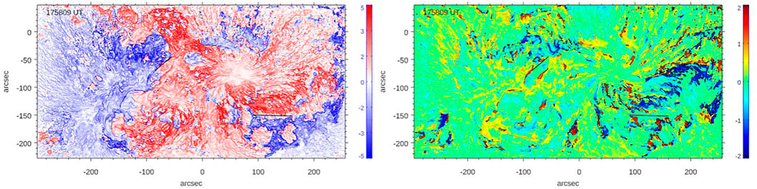
FIGURE 2. Distribution of log Q (left) and T_W parameters on the photosphere immediately before the flare onset. The two line segments in the maps mark strong Q-lanes situated above the photospheric polarity inversion line. The T_W image is scaled between − 2 < T_W < 2, while contours outline areas with |T_W| > 1.

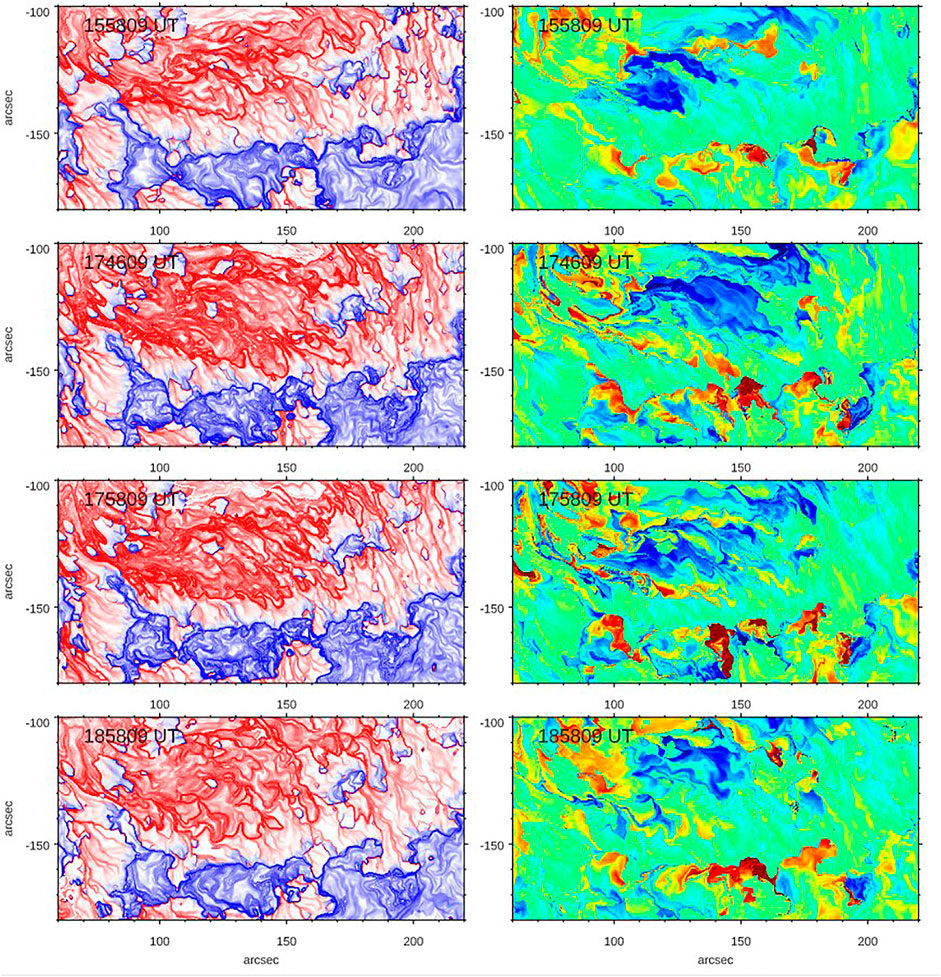
FIGURE 3. Evolution of Q (left) and T_W parameters near the flaring PIL. Twist maps are scaled between ±2 units.

To explore the evolution of coronal fields above the flaring PIL, we calculated T_W maps (Figure 4) at a vertical plane crossing the system of intertwining lines in its mid-section (x = 100, y = −120 to −170, see white vertical line in Figure 1). The leading sunspot was located to the left of the FOV (x = −15^″) and the sunspot field manifested itself in the upper part of the panels as diagonally slanted narrow islands of positive and negative twist patches. There were two time intervals (09:00-16:00 UT and 16:00-19:00 UT) during which various large twist structures formed and disappeared. About 2 hs prior to the flare (15:58:09 UT panel) there were no strong twist structures present above the PIL located at x = 25^″, and only one positive T_W patch was detected $\approx 10^{″}$ above the photosphere south of the PIL at x = 39^″. Note, that the origin of the x-axis is at the upper tip of the white line segment in Figure 1. According to the 17:46:09 UT panel in Figure 4, this structure at that time significantly weakened which is also reflected in the narrowing of the weak Q-corridor discussed above. By 17:20 UT a patch of T_W > 1 (blue) has developed in the center of the FOV surrounded by an extended area of positively twisted fields (red). It was later (17:58 UT) seen weakened and elongated as it was rising up into the corona. At the same time, many strongly twisted structures seen below y = 10^″ in the 17:58 UT panel have disappeared from the FOV as well. We also note that the strongly positively twisted structure with T_W > 2 seen at (40^″, 10^″) observed at 16:00 UT remained stationary during as well as after the eruption.

FIGURE 4. Field line twist, T_W, maps shown for several instances for the west flux rope (FR). The T_W was calculated on a vertical plane orthogonal to the axis of an eruptive AR filament. The images are scaled between − 2 < T_W < 2, while contours outline areas with |T_W| > 1. The black curve is the decay index profile calculated along the flaring PIL at x = 25^″. The x-axis begins at the top end of the cross-section (Figure 1) and the sunspot is outside the FOV on the left side of the panels. The y-axis represents the height above the photosphere. The color coded dots in 17:46:09 and 18:58:09 UT panels indicate the locations through which we traced the fields lines shown in Figure 5.

In Figure 5 we show line plots for the pre(17:46 UT, top) and post eruption (18:58 UT, bottom) models. Different colors indicate different magnetic flux systems. The choice of plotted field lines was dictated by the twist structures shown in the 17:46:09 UT and 18:58:09 UT panels in Figure 4. To visualize the 3D structures associated with the 2D twist patches we manually selected pixels in these panels through which we intended to trace field lines. As a rule, the pixels were selected to outline twist patches of interests including several trace points within a patch. Thus, the white-blue colored field lines in panel c are those that pass through the negative (blue) T_W patch centered at (30^″, 25^″) in the 17:46:09 UT panel, while the green colored lines are associated with the positive (red) patch at (20^″, 23^″). Similarly, the dark red lines are associated with the strong positive T_W at (40^″, 10^″) and the purple lines are those passing through two small scale patches seen below 10^″. The left column of panels shows side views of the same line plot. Panel b (axis view) shows that most of the red field lines make at least one turn, although when inspecting all panels together one may arrive to a conclusion that some of the red lines make two turns: first they dip and turn under the green and orange lines in the right side of the panels and then they make another turn in the left side of the panel. Some of the green lines, too, dip and turn under the orange and red lines and then continue as a large loop. They (green lines) are also seen in panel b making a full turn. The pink lines appear be less twisted and only some of them are likely to make one turn, thus representing a weakly twisted MFR (Patsourakos et al., 2020). The bottom set of panels in Figure 5 show the field lines extrapolated using an after-flare 18:58:09 UT HMI magnetogram. The flare-related reconfiguration of the magnetic fields is evident in both the twist and the line plot images. The only structure least affected by the flare is the MFR seen at (40^″, 10^″) in the T_W panel (dark red lines). The overlying fields (blue, green) seemingly changed their connectivity and appear now less twisted, while the twisted bundle of green, red and purple lines in the center of the upper-right panel and the corresponding T_w structures have disappeared and the overall configuration became more relaxed. These extrapolation results suggest that the photosphere “sensed” the eruption which manifested itself in restructuring of coronal fields.

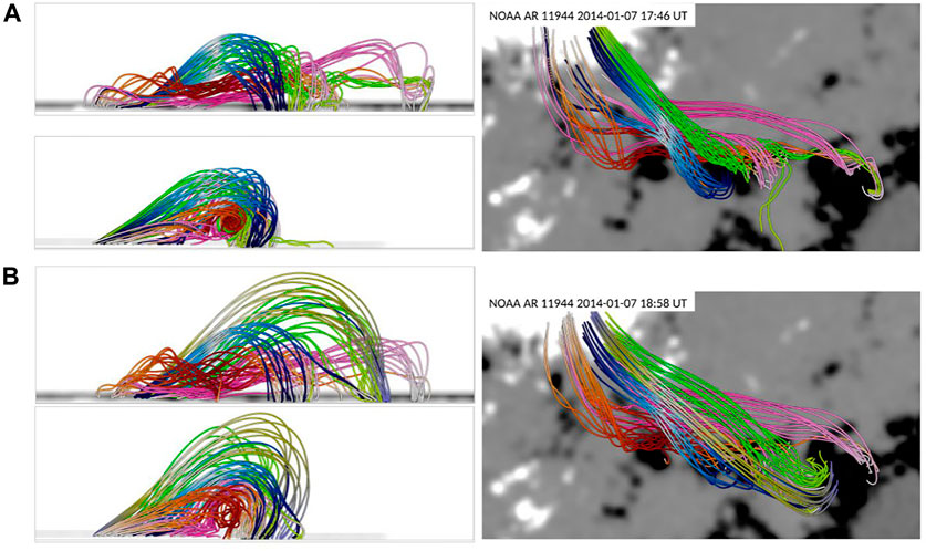
FIGURE 5. Results of magnetic field extrapolation using a pre-flare 17:46 UT, (A) and post-flare 18:58 UT, (B) magnetic field measurements. The FOV shown is 140 × 70 × 70″ and is located at 55 < x < 220 and − 180 < y < − 80 in Figure 1. Colored lines highlight various magnetic flux systems associated with the twist structures shown in Figure 4.

3.1 Decay Index and Critical Twist

Development of torus instability is mainly governed by the large-scale fields that straddle and stabilize a MFR. When the overlying fields sufficiently rapidly weaken with height, the MFR may become unstable and eruption may be initiated. The rate of decrease may be described by the decay index, n = −d log(B_ext)/d log(h) where B_ext and h are external potential field and height, (Kliem & Török, 2006), and it was suggested that configurations with n ≥ 1.5 are prone to torus instability (e.g., Török & Kliem, 2005; Aulanier et al., 2010). Following studies, however, reported that there may be a wide range of the eruption threshold values, 0.5 < n < 2, (e.g., Fan & Gibson, 2007; Démoulin & Aulanier, 2010; Olmedo & Zhang, 2010; Zuccarello et al., 2015; Jing et al., 2018).

In Figure 4 decay index profiles are plotter over the T_w images. The profiles were obtained by averaging individual profiles calculated along the line shown in Figures 1, 2 using potential field extrapolations. Instead of using the total perpendicular component of the potential field, we followed Kliem et al. (2021) recommendation and calculated the decay index only using the poloidal component of the potential field, which in our case, corresponds to the B_y component since the PIL runs parallel to the x-axis of the magnetogram. We should note though that we did calculate the decay index using the total horizontal field, and found that while there were no significant changes in the shape of the profiles, the values of the decay index were somewhat lower. The profiles show that the index began its steady decline at heights of about 23^″. However, its value remained below 1.5 level prior to and during the eruption, which is likely due to the strong sunspot fields extending above the flaring PIL. According to the model, the rising negative (blue) twist structure appeared to be sliding/escaping into the corona up and away from the leading sunspot along the sunspot field, thus suggesting that the associated coronal eruption and the CME may be deflected SW although the AR was located near the disk center. According to the CME Catalog (Yashiro et al., 2004) a massive halo CME² erupted at 18:24 UT with a linear speed of about 1830 km/s and mainly occupied the SW quadrant of the LASCO FOV, which qualitatively agrees with the above inference.

In contrast, similar T_W maps (Figure 6) made across the eastern PIL segment (see Figure 1) paint a far more stable picture where the main structural elements can be easily traced along the entire observed period. This area of the AR was associated only with frequent, short lived compact brightenings and it was not directly involved in the X1.2 flare discussed here. Nevertheless, the after flare 18:58 UT image shows that one of the positively twisted structures (red, at −30^″, 7^″) has disappeared from the FOV. The striking difference between the dynamics seen in these two cross-sections is also evidence that the evolution seen in Figure 4 is not due to inherent instabilities of the method, but are rather driven by varying photospheric boundary conditions.

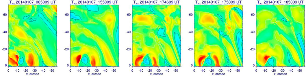
FIGURE 6. Field line twist, T_W, maps shown for several instances for the east flux rope (FR). The T_W was calculated on a vertical plane orthogonal to the eastern PIL. The images are scaled between − 2 < T_W < 2, while contours outline areas with |T_W| > 1. The x-axis begins at the upper-left end of the cross-section (Figure 1) and the sunspot is outside the FOV on the right side of the panels. The y-axis represents the height above the photosphere in arcsec.

3.2 Sign-Singularity Measure

We analysed the twist images by means of the sign-singularity measure, a function that displays a linear range with a slope of k, called cancellation exponent (Ott et al., 1992; Abramenko et al., 1998; Yurchyshyn et al., 2000a; Sorriso-Valvo et al., 2004; Yurchyshyn et al., 2012; Sorriso-Valvo et al., 2015). The dependence of the sign oscillation with spatial scale (scaling properties) can be analyzed by introducing the signed measure, χ(r), (Ott et al., 1992):

where U(x, y) is a studied signed parameter, and L_i(r) ⊂ L_i(R) represents a unique hierarchy of disjoint squares of size r, covering the whole square L of size R that encloses an AR of a part thereof (also see Yurchyshyn et al., 2000a, for details). We can then define a scaling exponent:

This measure allows us to analyse and qualitatively describe sign distribution and intensity fluctuations of a signed structure such as the twist images shown in Figure 4. Higher values of k (steeper measure) are only possible when the cancellations between positive and negative contributions in the sign-singular measure (hereafter called spectrum) reduce with r → 0, i.e., there is significant imbalance of the sign at all scales (for further discussion see Sorriso-Valvo et al., 2004). In general, an increase of the cancellation exponent indicates that the analyzed structure became either more fragmented (rapid fluctuation of sign) and/or the sign fluctuations become more powerful.

In Figure 7A we show χ(r) spectra calculated for T_W maps shown in Figure 4. The majority of the spectra in Figure 7A (except the 15:58 UT spectrum) do not show one extended linear range. Instead, the spectrum breaks in two intervals at scale of about 6 Mm, allowing us to determine two exponents, $k_T^{short}$ ($<6$Mm) and $k_T^{long}$ ($>6$Mm), and their variation over the observed period are shown in the right panel of Figure 7. There we also plot the total power, which is an integral of a spectrum over the entire spatial range. We see that the $k_T^{short}$ is very small and it does not show much time variations. The short scale end of the spectra below $<6$ Mm appears to be nearly saturated indicating that small-scale twist (current) structures below 6 Mm are rather smooth and devoid of significant fluctuations in sign. In contrast, the $k_T^{long}$ exponent is highly variable and is nearly synchronous with the total power, reflecting the varying height of the spectra (left panel). They both started to increase prior to a M7.2 flare that occurred in the trailing part of the AR. Although according to SDO/AIA data the M7.2 flare did not directly involve the studied area, it is worth noting that it was followed by multiple brightenings and plasma flows in the vicinity of both PILs. Nevertheless, the $k_T^{long}$ was steadily decreasing after this activity period and reached its minimum at about 16:00 UT, which can also be evidenced in Figure 4 as the large scale twist structures disappeared from the FOV between 14:00 UT and 16:00 UT. The $k_T^{long}$ and the total power began to increase again and peaked at about 17:30 UT, prior to the first short and compact brightenings that appeared at the eruption site. The twist images in Figure 4 show that during this time new large scale twist structures appeared, which then weakened and completely disappeared by the end of the impulsive phase of the flare (19:00 UT), which is also reflected in the $k_T^{long}$ and total power plots.

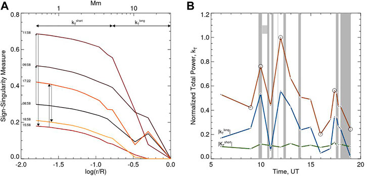
FIGURE 7. Sign-singularity measures (A), curves shown for selected time instances, and time variations of their parameters (B) calculated for the twist maps shown in Figure 4. In the (A) the arrows indicate direction of the evolution of these measures, while the time stamps are shown to connect these curves to the corresponding images in Figure 4. The two-sided arrows mark linear intervals used to calculate the cancellation exponent, $k_T^{short}$, and the slope of the long range end of the measure, $k_T^{long}$. (B) shows time variations of the total power (brown) calculated for each measure shown in the (A), as well as the corresponding cancellation exponent ($k_T^{short}$, green) and the slope ($k_T^{long}$, blue). The data points indicated by circles are those that correspond to the measures in the left plot. The vertical strips indicate the start time and the duration of AIA 17.1 nm brightenings and the X1.2 flare (18:00–19:00 UT) associated with the AR filament and the horizontal bar between 10:07 and 10:37 UT marks the timing of a M7.2 flare that occurred in the south-east part of the AR.

The $k_T^{long}$ exponent was determined from the model twist data and thus, in general, may not reflect real evolution of the AR magnetic fields. We thus utilized HMI magnetograms to calculate current helicity and the corresponding sign-singularity measures. Current helicity, H_c, defined as a product of the magnetic field and the associated electric currents. This parameter seems to be an important descriptor of energy capability of an AR (Seehafer, 1994). Some general characteristics of current helicity (such as imbalance, hemispherical segregation, injection rate, etc.) have been extensively studied by several groups (e.g., Pevtsov et al., 1994; Abramenko et al., 1996; Park et al., 2020). Abramenko et al. (1998) and Yurchyshyn et al. (2000b, 2012) studies showed that there is a noticeable decrease of the cancellation exponent prior to periods of enhanced flaring.

Similarly to the twist data, the $k_h^{short}$ exponent of current helicity (Figure 8A) does not show strong temporal variations and remains at ∼0.5 level for most of the time. The total power and $k_h^{long}$ exponent are synchronous and their general trend is similar to that observed for the twist parameter calculated for a vertical cross-section (Figures 4, 7, middle). They all peak at about 12:00 UT and at about 17:45 UT. In case of the X1.2 flare the cancellation exponent and the total power began their rapid decrease prior to the flare onset, which is consistent with the earlier reported findings and suggests that the magnetic configuration experienced rapid changes prior to the impulsive phase of the flare. We thus conclude that the modeled T_w maps and observed vector magnetograms seem to exhibit the same tendency, namely, enhancement of their structure prior to the flare and their rapid exhausting that begins immediately before the onset of the impulsive phase.

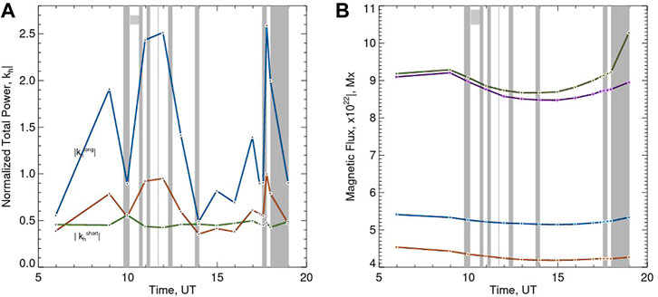
FIGURE 8. (A): Time variations of sign-singularity parameters calculated for current helicity maps obtained from observed vector magnetograms. The three curves show time variations of the total power (brown), the cancellation exponent ($k_T^{short}$, green), and the slope ($k_T^{long}$, blue). (B): Time variations of the magnitude of HMI magnetic flux calculated over the entire area shown in Figure 1. Blue and orange profiles show data for northward and southward B_z component, while green and purple profiles represent horizontal B_x and B_y flux. In both panels the vertical strips indicate the start time and the duration of AIA 17.1 nm brightenings and the X1.2 flare (18:00-19:00 UT) associated with the AR filament, while the horizontal bar between 10:07 and 10:37 UT marks the timing of a M7.2 flare that occurred in the east part of the AR.

In the right panel of Figure 8 we plot time variations of the total signed B_z, and unsigned B_x, and B_y flux calculated over the entire area shown in Figure 1. All four profiles exhibit coherent and gradual variations, which do not appear to be well correlated with the sign-singularity parameters showed in Figures 7, 8. The cancellation exponents peak twice at about 12:00 UT and 17:40 UT, when the magnetic flux was gradually decreasing (12:00 UT) and increasing (17:40 UT), while both cancellation exponents and magnetic flux have a wide minimum at about 14:00-16:00 UT. Therefore, while all profiles may show weakly correlated general trends, the strong peaks in the cancellation exponents may not be explained by rapid changes in the observed flux profiles.

4 Discussion and Conclusion

First, we summarize our main findings. Series of coronal field extrapolations suggest that 1) the pre-eruption configuration of the AR included several MFR-like structures with twist exceeding 2; we detected a well defined MFRs only at the site of the future eruption; 2) the eruption was affected by overlying sunspot fields, which caused the ejecta to deflect side-wise at the initial stage; 3) slide-out eruptions may explain a large spread of the eruption threshold of the decay index; 4) the photospheric and the corresponding extrapolated fields are sensitive to energy build up and release processes; 5) cancellation exponents calculated over the model twist data and the observed photospheric current helicity maps showed synchronous variations, which include pre-flare increase followed by a gradual decrease that begins with the flare onset.

Wang & Zhang (2007) found that confined, non-eruptive flares tend to originate from the magnetic center of ARs, while eruptive ones are more likely to erupt from the periphery of ARs. These results emphasise the role that overlying fields play in producing CMEs (see also Baumgartner et al., 2018). Panasenco et al. (2013) reported that during the eruption process the ejected magnetic fields are channeled toward weaker fields, which facilitates their escape from the corona. Thus, coronal holes or sunspot fields may create unbalanced forces acting on an ejecta (e.g., Gopalswamy et al., 2009) causing them to propagate in the non-radial direction along a path with least resistance, which is away from a coronal hole or a sunspot. On the other hand, magnetic fields of AR 11943, located immediately west of the studied AR, appear to be connected to the eruption site as evidenced by several initial flare brightening that occurred at the interface between the two ARs. It may be speculated that this pre-flare activity was a manifestation of reconnection processes that may have weakened the strapping fields and created favourable conditions for channeling and deflecting the resulting CME.

Very recently Kliem et al. (2021) arrived to a similar conclusion analyzing a height profile of a decay index calculated along an oblique propagation direction. In our case, the vertical decay index exceeded n = 1 value only at heights above 50^″, which corresponded to the slanted sunspot fields, while the top of the large T_W structures reached heights of about 35^″. Although we did not calculate the oblique decay index, combination of the decay index profiles and twist maps allowed us to speculate that at heights above 30^″ the decay index along the presumed propagation channel would decrease more rapidly thus facilitating the eruption process. It should be noted that earlier studies reported a wide range of the eruption threshold values, 0.5 < n < 2, (e.g., Fan & Gibson, 2007; Démoulin & Aulanier, 2010; Olmedo & Zhang, 2010; Zuccarello et al., 2015; Jing et al., 2018). The oblique eruption process, discussed above, may partially account for the wide range of eruption thresholds. Another possible reason is that the critical decay index was derived from a rather simple model. At the same time, the critical value is strongly dependent on the boundary conditions, aspect ratio of the MFR, other parameters (e.g., Alt et al., 2021). The MFR derived from our extrapolations represents a very complex structure and it is likely that lower values of the decay index are allowed as the critical value. For example, Inoue et al. (2016) concluded that if multiple MFR are present and some of them have the same helicity, then the pinch force will make the system more stable, which of course will modify the critical value of the decay index. Finally, Ishiguro & Kusano (2017) found that a double arc loop system may become unstable even if the external field does not decay with altitude. Thus the double arc instability (Ishiguro & Kusano, 2017), being independent of the decay index, may realize conditions for tether-cutting reconnection as an onset mechanism of solar eruptions.

Wang et al. (2015) analyzed the same AR as that studied here and argued that open field structures detected in their extrapolations could be a guide for the eruption fields (see also Möstl et al., 2015). Our extrapolations did not include open field lines at the site of the eruption, however, we note that Fleishman et al. (2019) concluded that the NLFFF extrapolation routine tends to produce a more “closed” magnetic field configuration as compared to the test data. We therefore speculate that the ejecta was non-radially escaping from underneath the extended sunspot fields, along a channel with a low decay index. Although details of our and Wang et al. (2015) extrapolations may differ, they both agree on the non-radial propagation of the ejecta and strong influence of the sunspot fields. We thus further confirm the important role that the large scale magnetic environment play in the low corona in defining the direction of a magnetic eruption. An alternative explanation of the CME deflection may be a medium-sized coronal hole that was located approximately at 0.5 solar roadii north-east of the AR. It is known that coronal hole may deflect CMEs (e.g., Gopalswamy et al., 2009), although this coronal hole appeared to be too far to have a dominant effect at the early stage of the eruption.

Zheng et al. (2016) suggested that the complex structure of the X1.2 flare in AR NOAA 11944 may result from a complex distribution of photospheric magnetic flux and that the eruption probably involved at least two magnetic reconnection events. These inferences are in accord with our model data, which show presence of several MFRs nested above the PIL. While we did not consider details of magnetic restructuring and possible changes in MFR footpoint connectivity that led to the eruption, it is safe to assume that eruption of these complex structures may, at least partially, explain the complex structure of flare emission. This is also in line with Kliem et al. (2021) arguments that an unstable MFR may be formed or enhanced by a series of confined flares prior to complete eruption. It subsequent evolution toward an equilibrium state may explain the slow-rise stage of an ejecta. Here we would like to note that, according to the field extrapolations, significant changes in the corona of the AR commenced at approximately 17:46 UT, i.e., 15 min prior to the X1.2 flare onset. During this pre-flare activation period, various plasma flows and compact burst like brightenings were detected in AIA 17.1 nm data, while the impulsive phase of the eruption with enhanced emission began only after 18:00 UT. We may speculate that the pre-flare changes seen in the model field and driven by observed photospheric magnetograms may be the search of the equilibrium suggested by Kliem et al. (2021).

Pre-flare changes in the magnetic fields are also evident in the sign-singularity analysis that show enhancements of model twist and observed current helicity structures prior to the flare followed by their rapid exhaust during the pre-flare activation period. These findings are in agreement with our earlier studies based on data with lower spatial and temporal resolution, which indicated that current helicity distribution may rapidly change prior to a flare event (Abramenko et al., 1998; Yurchyshyn et al., 2000a, 2012). Since the magnetic flux plots do not show any variations that would temporarily correlate with the cancellation exponents, we may suggest that the structural variations in the AR were mostly associated with enhancements of current systems (twist) in the AR rather than energy injection via new flux emergence.

According to the model data, strong twist structures developed in the AR corona within several hours prior to the eruption. It is not clear what was the driver of this pre-flare energy build up above the PIL. The eruption occurred at the periphery of the AR and HMI magnetograms did not show any evidence of new magnetic flux emerging in the area. The Q-maps in Figure 3 and the local correlation tracking technique indicated that there were converging motions toward the flaring PIL. We therefore speculate that the most likely mechanism responsible for the origin of the pre-flare MFR build-up detected in the model data is magnetic reconnection resulting from restructuring of the AR magnetic fields driven by the converging flows as well as the series of small flares east of the eruption site. Although this assumption agrees with the occurrence of multiple brightenings prior to the onset of the main flare, a in depth study and MHD simulations are needed to understand this process. It is also worth noting that this process may also be considered as condensation of magnetic helicity at PILs (Antiochos, 2013). It is proposed that helicity is injected into the AR atmosphere by the continuous large and small-scale photospheric motions and flux emergence and it may then be cascading toward larger spatial scales. It is thus plausible that rapid formation of large twist structures seen in the extrapolated data are due to transfer of “pre-existing” helicity from small to large-scale structures via magnetic reconnection, which conserves the helicity present in a given domain (Berger, 1984).

Finally, this study demonstrates that coronal models of AR magnetic fields may have a potential for predicting likelihood, location, and timing of solar flares. Thus, analysis of coronal configurations using available extrapolation tools (e.g., Wiegelmann et al., 2006; Fleishman et al., 2017; Duan et al., 2019; Fleishman et al., 2019) and/or MHD modeling (e.g., Cheung & DeRosa, 2012; Jiang & Feng, 2012; Inoue et al., 2014; Jiang et al., 2016) may reveal the existence and location of a MFR in an AR, while time profiles of various parameters describing magnetic fields structures may be utilized to study timing of ongoing evolution. Very recently, Gupta et al. (2021) studied relative magnetic helicity variations for a sample of ten ARs that produced large solar flares (GOES class $>$ M1.0) using NLFFF extrapolations produced by Wiegelmann & Inhester (2010) method. In particular they note that energy and helicity ratios derived from NLFFF data may allow us to determine the potential of an AR to produce a CME.

Data Availability Statement

Publicly available datasets were analyzed in this study. This data can be found here: http://jsoc.stanford.edu/ajax/exportdata.html.

Author Contributions

VY is the leader of the study and he proposed the original idea, XY performed simulations, GN and GF developed the gx_simulator, VA developed the sign-singularity method, SI assisted in interpretation of simulated data and the decay index, E-KL and WC contributed to interpretation of the observed data and results.

Funding

BBSO operation is supported by NJIT and US NSF AGS-1821294 grants. GST operation is partly supported by the Korea Astronomy and Space Science Institute (KASI), and Seoul National University. This work was supported in part by NSF grants AST-1820613, AGS-1927578, AGS-1743321, and AGS-2121632, and NASA grants 80NSSC18K0667, 80NSSC19K0068, and 80NSSC20K0627 awarded to NJIT. VY acknowledges support from NSF AST-1614457, AGS-1954737, AST-2108235, AFOSR FA9550-19-1-0040, NASA 80NSSC17K0016, 80NSSC19K0257, and 80NSSC20K0025 grants.

Conflict of Interest

The authors declare that the research was conducted in the absence of any commercial or financial relationships that could be construed as a potential conflict of interest.

Publisher’s Note

All claims expressed in this article are solely those of the authors and do not necessarily represent those of their affiliated organizations, or those of the publisher, the editors and the reviewers. Any product that may be evaluated in this article, or claim that may be made by its manufacturer, is not guaranteed or endorsed by the publisher.

Acknowledgments

We thank referees for careful reading the manuscript and providing valuable criticism and suggestions.

Footnotes

¹ftp://gong2.nso.edu/HA/hag/201401/20140107/

²https://cdaw.gsfc.nasa.gov/CME_list/UNIVERSAL/2014_01/univ2014_01.html

References

Abramenko, V. I., Wang, T., and Yurchishin, V. B. (1996). Analysis of Electric Current Helicity in Active Regions on the Basis of Vector Magnetograms. Sol. Phys. 168, 75–89. doi:10.1007/BF00145826
Alt, A., Myers, C. E., Ji, H., Jara-Almonte, J., Yoo, J., Bose, S., et al. (2021). Laboratory Study of the Torus Instability Threshold in Solar-Relevant, Line-Tied Magnetic Flux Ropes. Astrophysical J. 908, 41. doi:10.3847/1538-4357/abda4b
Antiochos, S. K., DeVore, C. R., and Klimchuk, J. A. (1999). A Model for Solar Coronal Mass Ejections. Astrophysical J. 510, 485–493. doi:10.1086/306563
Antiochos, S. K. (2013). Helicity Condensation as the Origin of Coronal and Solar Wind Structure. Astrophysical J. 772, 72. doi:10.1088/0004-637X/772/1/72
Aulanier, G., Török, T., Démoulin, P., and DeLuca, E. E. (2009). Formation of Torus-Unstable Flux Ropes and Electric Currents in Erupting Sigmoids. Astrophysical J. 708, 314–333. doi:10.1088/0004-637x/708/1/314
Aulanier, G., Török, T., Démoulin, P., and DeLuca, E. E. (2010). Formation of Torus-Unstable Flux Ropes and Electric Currents in Erupting Sigmoids. Astrophysical J. 708, 314–333. doi:10.1088/0004-637X/708/1/314
Barnes, G., Leka, K. D., Schrijver, C. J., Colak, T., Qahwaji, R., Ashamari, O. W., et al. (2016). A Comparison of Flare Forecasting Methods. I. Results from the "All-clear" Workshop. Astrophysical J. 829, 89. doi:10.3847/0004-637x/829/2/89
Baty, H. (2001). On the MHD Stability of the $\vec M$ = 1 Kink Mode in Solar Coronal Loops. Astron. Astrophysics 367, 321–325. doi:10.1051/0004-6361:20000412
Baumgartner, C., Thalmann, J. K., and Veronig, A. M. (2018). On the Factors Determining the Eruptive Character of Solar Flares. Astrophysical J. 853, 105. doi:10.3847/1538-4357/aaa243
Berger, M. A., and Prior, C. (2006). The Writhe of Open and Closed Curves. J. Phys. A: Math. Gen. 39, 8321–8348. doi:10.1088/0305-4470/39/26/005
Berger, M. A. (1984). Rigorous New Limits on Magnetic Helicity Dissipation in the Solar corona. Geophys. Astrophysical Fluid Dyn. 30, 79–104. doi:10.1080/03091928408210078
Bobra, M. G., Sun, X., Hoeksema, J. T., Turmon, M., Liu, Y., Hayashi, K., et al. (2014). The Helioseismic and Magnetic Imager (HMI) Vector Magnetic Field Pipeline: SHARPs - Space-Weather HMI Active Region Patches. Sol. Phys. 289, 3549–3578. doi:10.1007/s11207-014-0529-3
Burlaga, L., Sittler, E., Mariani, F., and Schwenn, R. (1981). Magnetic Loop behind an Interplanetary Shock: Voyager, Helios, and IMP 8 Observations. J. Geophys. Res. 86, 6673. doi:10.1029/JA086iA08p06673
Chen, P. F., and Shibata, K. (2000). An Emerging Flux Trigger Mechanism for Coronal Mass Ejections. Astrophysical J. 545, 524–531. doi:10.1086/317803
Cheung, M. C. M., and DeRosa, M. L. (2012). A Method for Data-Driven Simulations of Evolving Solar Active Regions. Astrophysical J. 757, 147. doi:10.1088/0004-637X/757/2/147
Démoulin, P., and Aulanier, G. (2010). Criteria for Flux Rope Eruption: Non-equilibrium versus Torus Instability. Astrophysical J. 718, 1388–1399. doi:10.1088/0004-637X/718/2/1388
D. Fleishman, G., Anfinogentov, S., Loukitcheva, M., Mysh’yakov, I., and Stupishin, A. (2017). Casting the Coronal Magnetic Field Reconstruction Tools in 3D Using the MHD Bifrost Model. Astrophysical J. 839, 30. doi:10.3847/1538-4357/aa6840
Duan, A., Jiang, C., He, W., Feng, X., Zou, P., and Cui, J. (2019). A Study of Pre-flare Solar Coronal Magnetic Fields: Magnetic Flux Ropes. Astrophysical J. 884, 73. doi:10.3847/1538-4357/ab3e33
Duan, A., Jiang, C., Zou, P., Feng, X., and Cui, J. (2021). Structure and Evolution of an Inter-active Region Large-Scale Magnetic Flux Rope. JThe Astrophysical J. 906, 45. doi:10.3847/1538-4357/abc701
Falconer, D. A., Moore, R. L., Barghouty, A. F., and Khazanov, I. (2014). MAG4 versus Alternative Techniques for Forecasting Active Region Flare Productivity. Space Weather 12, 306–317. doi:10.1002/2013SW001024
Falconer, D. A., Tiwari, S. K., Moore, R. L., and Khazanov, I. (2016). A New Method to Quantify and Reduce the Net Projection Error in Whole-Solar-Active-Region Parameters Measured from Vector Magnetograms. Astrophysical J. 833, L31. doi:10.3847/2041-8213/833/2/L31
Fan, Y., and Gibson, S. E. (2004). Numerical Simulations of Three‐dimensional Coronal Magnetic Fields Resulting from the Emergence of Twisted Magnetic Flux Tubes. Astrophysical J. 609, 1123–1133. doi:10.1086/421238
Fan, Y., and Gibson, S. E. (2007). Onset of Coronal Mass Ejections Due to Loss of Confinement of Coronal Flux Ropes. Astrophysical J. 668, 1232–1245. doi:10.1086/521335
Fan, Y., and Gibson, S. E. (2003). The Emergence of a Twisted Magnetic Flux Tube into a Preexisting Coronal Arcade. Astrophysical J. 589, L105–L108. doi:10.1086/375834
Fleishman, G., Mysh’yakov, I., Stupishin, A., Loukitcheva, M., and Anfinogentov, S. (2019). Force-free Field Reconstructions Enhanced by Chromospheric Magnetic Field Data. Astrophysical J. 870, 101. doi:10.3847/1538-4357/aaf384
Gopalswamy, N., Mäkelä, P., Xie, H., Akiyama, S., and Yashiro, S. (2009). CME Interactions with Coronal Holes and Their Interplanetary Consequences. J. Geophys. Res. 114, a–n. doi:10.1029/2008JA013686
Gopalswamy, N., Yashiro, S., and Akiyama, S. (2007). Geoeffectiveness of Halo Coronal Mass Ejections. J. Geophys. Res. 112, a–n. doi:10.1029/2006JA012149
Gosling, J. T., Bame, S. J., McComas, D. J., and Phillips, J. L. (1990). Coronal Mass Ejections and Large Geomagnetic Storms. Geophys. Res. Lett. 17, 901–904. doi:10.1029/GL017i007p00901
Gupta, M., Thalmann, J. K., and Veronig, A. M. (2021). arXiv E-Prints, arXiv:2106.08781. arXiv:2106.08781. Available at: https://arxiv.org/abs/2106.08781.
Hood, A. W., and Priest, E. R. (1981). Critical Conditions for Magnetic Instabilities in Force-free Coronal Loops. Geophys. Astrophysical Fluid Dyn. 17, 297–318. doi:10.1080/03091928108243687
Inoue, S., Hayashi, K., and Kusano, K. (2016). Structure and Stability of Magnetic Fields in Solar Active Region 12192 Based on Nonlinear Force-free Field Modeling. Astrophysical J. 818, 168. doi:10.3847/0004-637X/818/2/168
Inoue, S., Magara, T., Pandey, V. S., Shiota, D., Kusano, K., Choe, G. S., et al. (2014). Nonlinear Force-free Extrapolation of the Coronal Magnetic Field Based on the Magnetohydrodynamic Relaxation Method. Astrophysical J. 780, 101. doi:10.1088/0004-637X/780/1/101
Ishiguro, N., and Kusano, K. (2017). Double Arc Instability in the Solar Corona. Astrophysical J. 843, 101. doi:10.3847/1538-4357/aa799b
Jiang, C., and Feng, X. (2012). A New Implementation of the Magnetohydrodynamics-Relaxation Method for Nonlinear Force-free Field Extrapolation in the Solar Corona. Astrophysical J. 749, 135. doi:10.1088/0004-637X/749/2/135
Jiang, C., Wu, S. T., Yurchyshyn, V., Wang, H., Feng, X., and Hu, Q. (2016). How Did a Major Confined Flare Occur in Super Solar Active Region 12192? Astrophysical J. 828, 62. doi:10.3847/0004-637X/828/1/62
Jing, J., Liu, C., Lee, J., Ji, H., Liu, N., Xu, Y., et al. (2018). Statistical Analysis of Torus and Kink Instabilities in Solar Eruptions. Astrophysical J. 864, 138. doi:10.3847/1538-4357/aad6e4
Karpen, J. T., Antiochos, S. K., and DeVore, C. R. (2012). The Mechanisms for the Onset and Explosive Eruption of Coronal Mass Ejections and Eruptive Flares. Astrophysical J. 760, 81. doi:10.1088/0004-637x/760/1/81
Kliem, B., Lee, J., Liu, R., White, S. M., Liu, C., and Masuda, S. (2021). Nonequilibrium Flux Rope Formation by Confined Flares Preceding a Solar Coronal Mass Ejection. Astrophysical J. 909, 91. doi:10.3847/1538-4357/abda37
Kliem, B., and Török, T. (2006). Torus Instability. Phys. Rev. Lett. 96, 255002. doi:10.1103/physrevlett.96.255002
Kusano, K., Bamba, Y., Yamamoto, T. T., Iida, Y., Toriumi, S., and Asai, A. (2012). Magnetic Field Structures Triggering Solar Flares and Coronal Mass Ejections. Astrophysical J. 760, 31. doi:10.1088/0004-637X/760/1/31
Kusano, K., Iju, T., Bamba, Y., and Inoue, S. (2020). A Physics-Based Method that Can Predict Imminent Large Solar Flares. Science 369, 587–591. doi:10.1126/science.aaz2511
Leka, K. D., Park, S.-H., Kusano, K., Andries, J., Barnes, G., Bingham, S., et al. (2019a). A Comparison of Flare Forecasting Methods. II. Benchmarks, Metrics, and Performance Results for Operational Solar Flare Forecasting Systems. Astrophysical J. 243, 36. doi:10.3847/1538-4365/ab2e12
Leka, K. D., Park, S.-H., Kusano, K., Andries, J., Barnes, G., Bingham, S., et al. (2019b). A Comparison of Flare Forecasting Methods. III. Systematic Behaviors of Operational Solar Flare Forecasting Systems. Astrophysical J. 881, 101. doi:10.3847/1538-4357/ab2e11
Lemen, J. R., Title, A. M., Akin, D. J., Boerner, P. F., Chou, C., Drake, J. F., et al. (2012). The Atmospheric Imaging Assembly (AIA) on the Solar Dynamics Observatory (SDO). Solar Phys. 275, 17. doi:10.1007/s11207-011-9776-8
Liu, R., Kliem, B., Titov, V. S., Chen, J., Wang, Y., Wang, H., et al. (2016). Structure, Stability, and Evolution of Magnetic Flux Ropes from the Perspective of Magnetic Twist. Astrophysical J. 818, 148. doi:10.3847/0004-637X/818/2/148
Lu, Z., Cao, W., Jin, G., Zhang, Y., Ding, M., and Guo, Y. (2019). A Statistical Study of the Magnetic Imprints of X-Class Solar Flares. Astrophysical J. 876, 133. doi:10.3847/1538-4357/ab16d4
Marubashi, K., Akiyama, S., Yashiro, S., Gopalswamy, N., Cho, K.-S., and Park, Y.-D. (2015). Geometrical Relationship between Interplanetary Flux Ropes and Their Solar Sources. Sol. Phys. 290, 1371–1397. doi:10.1007/s11207-015-0681-4
Moore, R. L., Sterling, A. C., Hudson, H. S., and Lemen, J. R. (2001). Onset of the Magnetic Explosion in Solar Flares and Coronal Mass Ejections. Astrophysical J. 552, 833–848. doi:10.1086/320559
Möstl, C., Rollett, T., Frahm, R. A., Liu, Y. D., Long, D. M., Colaninno, R. C., et al. (2015). Strong Coronal Channelling and Interplanetary Evolution of a Solar Storm up to Earth and Mars. Nat. Commun. 6, 7135. doi:10.1038/ncomms8135
Nita, G. M., Fleishman, G. D., Kuznetsov, A. A., Kontar, E. P., and Gary, D. E. (2015). Three-dimensional Radio and X-ray Modeling and Data Analysis Software: Revealing Flare Complexity. Astrophysical J. 799, 236. doi:10.1088/0004-637X/799/2/236
Nita, G. M., Viall, N. M., Klimchuk, J. A., Loukitcheva, M. A., Gary, D. E., Kuznetsov, A. A., et al. (2018). Dressing the Coronal Magnetic Extrapolations of Active Regions with a Parameterized Thermal Structure. Astrophysical J. 853, 66. doi:10.3847/1538-4357/aaa4bf
Olmedo, O., and Zhang, J. (2010). Partial Torus Instability. Astrophysical J. 718, 433–440. doi:10.1088/0004-637X/718/1/433
Ott, E., Du, Y., Sreenivasan, K. R., Juneja, A., and Suri, A. K. (1992). Sign-singular Measures: Fast Magnetic Dynamos, and high-Reynolds-number Fluid Turbulence. Phys. Rev. Lett. 69, 2654–2657. doi:10.1103/PhysRevLett.69.2654
Panasenco, O., Martin, S. F., Velli, M., and Vourlidas, A. (2013). Origins of Rolling, Twisting, and Non-radial Propagation of Eruptive Solar Events. Sol. Phys. 287, 391–413. doi:10.1007/s11207-012-0194-3
Park, S.-H., Leka, K. D., Kusano, K., Andries, J., Barnes, G., Bingham, S., et al. (2020). A Comparison of Flare Forecasting Methods. IV. Evaluating Consecutive-Day Forecasting Patterns. Astrophysical J. 890, 124. doi:10.3847/1538-4357/ab65f0
Patsourakos, S., Vourlidas, A., Török, T., Kliem, B., Antiochos, S. K., Archontis, V., et al. (2020). Decoding the Pre-eruptive Magnetic Field Configurations of Coronal Mass Ejections. Space Sci. Rev. 216, 131. doi:10.1007/s11214-020-00757-9
Pesnell, W. D., Thompson, B. J., and Chamberlin, P. C. (2012). The Solar Dynamics Observatory (SDO). Sol. Phys. 275, 3–15. doi:10.1007/s11207-011-9841-3
Pevtsov, A. A., Canfield, R. C., and Metcalf, T. R. (1994). Patterns of Helicity in Solar Active Regions. Astrophysical J. 425, L117. doi:10.1086/187324
Pevtsov, A. A., and Canfield, R. C. (2001). Solar Magnetic fields and Geomagnetic Events. J. Geophys. Res. 106, 25191–25197. doi:10.1029/2000JA004018
Savcheva, A., Pariat, E., van Ballegooijen, A., Aulanier, G., and DeLuca, E. (2012). Sigmoidal Active Region on the Sun: Comparison of a Magnetohydrodynamical Simulation and a Nonlinear Force-free Field Model. Astrophysical J. 750, 15. doi:10.1088/0004-637x/750/1/15
Scherrer, P. H., Schou, J., Bush, R. I., Kosovichev, A. G., Bogart, R. S., Hoeksema, J. T., et al. (2012). The Helioseismic and Magnetic Imager (HMI) Investigation for the Solar Dynamics Observatory (SDO). Sol. Phys. 275, 207–227. doi:10.1007/s11207-011-9834-2
Schou, J., Scherrer, P. H., Bush, R. I., Wachter, R., Couvidat, S., Rabello-Soares, M. C., et al. (2012). Design and Ground Calibration of the Helioseismic and Magnetic Imager (HMI) Instrument on the Solar Dynamics Observatory (SDO). Solar Phys. 275, 229. doi:10.1007/s11207-011-9842-2
Sorriso-Valvo, L., Carbone, V., Veltri, P., Abramenko, V. I., Noullez, A., Politano, H., et al. (2004). Topological Changes of the Photospheric Magnetic Field inside Active Regions: A Prelude to Flares? Planet. Space Sci. 52, 937–943. doi:10.1016/j.pss.2004.02.006
Sorriso-Valvo, L., De Vita, G., Kazachenko, M. D., Krucker, S., Primavera, L., Servidio, S., et al. (2015). Sign Singularity and Flares in Solar Active Region Noaa 11158. Astrophysical J. 801, 36. doi:10.1088/0004-637X/801/1/36
Srivastava, N., and Venkatakrishnan, P. (2004). Solar and Interplanetary Sources of Major Geomagnetic Storms during 1996-2002. J. Geophys. Res. 109, A10103. doi:10.1029/2003JA010175
Thompson, W. T. (2006). Coordinate Systems for Solar Image Data. Astron. Astrophysics 449, 791–803. doi:10.1051/0004-6361:20054262
Titov, V. S. (2007). Generalized Squashing Factors for Covariant Description of Magnetic Connectivity in the Solar Corona. Astrophysical J. 660, 863–873. doi:10.1086/512671
Titov, V. S., Hornig, G., and Démoulin, P. (2002). Theory of Magnetic Connectivity in the Solar corona. J. Geophys. Res. 107, 3–1. doi:10.1029/2001JA000278
Toriumi, S., Schrijver, C. J., Harra, L. K., Hudson, H., and Nagashima, K. (2017). Magnetic Properties of Solar Active Regions that Govern Large Solar Flares and Eruptions. Astrophysical J. 834, 56. doi:10.3847/1538-4357/834/1/56
Toriumi, S., and Takasao, S. (2017). Numerical Simulations of Flare-Productive Active Regions:δ-Sunspots, Sheared Polarity Inversion Lines, Energy Storage, and Predictions. Astrophysical J. 850, 39. doi:10.3847/1538-4357/aa95c2
Török, T., and Kliem, B. (2005). Confined and Ejective Eruptions of Kink-Unstable Flux Ropes. Astrophysical J. 630, L97–L100. doi:10.1086/462412
Török, T., and Kliem, B. (2003). The Evolution of Twisting Coronal Magnetic Flux Tubes. Astron. Astrophysics 406, 1043–1059. doi:10.1051/0004-6361:20030692
Tsurutani, B. T., Gonzalez, W. D., Tang, F., Akasofu, S. I., and Smith, E. J. (1988). Origin of Interplanetary Southward Magnetic fields Responsible for Major Magnetic Storms Near Solar Maximum (1978-1979). J. Geophys. Res. 93, 8519. doi:10.1029/JA093iA08p08519
Wang, R., Liu, Y. D., Dai, X., Yang, Z., Huang, C., and Hu, H. (2015). The Role of Active Region Coronal Magnetic Field in Determining Coronal Mass Ejection Propagation Direction. Astrophysical J. 814, 80. doi:10.1088/0004-637X/814/1/80
Wang, Y., and Zhang, J. (2007). A Comparative Study between Eruptive X‐Class Flares Associated with Coronal Mass Ejections and Confined X‐Class Flares. Astrophysical J. 665, 1428–1438. doi:10.1086/519765
Wheatland, M. S., Sturrock, P. A., and Roumeliotis, G. (2000). An Optimization Approach to Reconstructing Force‐free Fields. Astrophysical J. 540, 1150–1155. doi:10.1086/309355
Wiegelmann, T., and Inhester, B. (2010). How to deal with Measurement Errors and Lacking Data in Nonlinear Force-free Coronal Magnetic Field Modelling? Astron. Astrophysics 516, 516A107. doi:10.1051/0004-6361/201014391
Wiegelmann, T., Inhester, B., and Sakurai, T. (2006). Preprocessing of Vector Magnetograph Data for a Nonlinear Force-free Magnetic Field Reconstruction. Sol. Phys. 233, 215–232. doi:10.1007/s11207-006-2092-z
Wiegelmann, T. (2004). Optimization Code with Weighting Function for the Reconstruction of Coronal Magnetic fields. Solar Phys. 219, 87–108. doi:10.1023/B:SOLA.0000021799.39465.36
Yardley, S. L., Mackay, D. H., and Green, L. M. (2021). Simulating the Coronal Evolution of Bipolar Active Regions to Investigate the Formation of Flux Ropes. Sol. Phys. 296, 10. doi:10.1007/s11207-020-01749-2
Yashiro, S., Gopalswamy, N., Michalek, G., St. Cyr, O. C., Plunkett, S. P., Rich, N. B., et al. (2004). A Catalog of white Light Coronal Mass Ejections Observed by the SOHO Spacecraft. J. Geophys. Res. (Space Physics) 109, A07105. doi:10.1029/2003JA010282
Yurchyshyn, V., Abramenko, V., and Watanabe, H. (2012). “Astronomical Society of the Pacific Conference Series,” in Hinode-3: The 3rd Hinode Science Meeting. Editors T. Sekii, T. Watanabe, and T. Sakurai, Vol. 454, 311.
Yurchyshyn, V. B., Abramenko, V. I., and Carbone, V. (2000a). Flare‐Related Changes of an Active Region Magnetic Field. Astrophysical J. 538, 968–979. doi:10.1086/309139
Yurchyshyn, V. B., Abramenko, V. I., and Carbone, V. (2000b). Flare‐Related Changes of an Active Region Magnetic Field. Astrophysical J. 538, 968–979. doi:10.1086/309139
Yurchyshyn, V., Hu, Q., and Abramenko, V. (2005). Structure of Magnetic fields in NOAA Active Regions 0486 and 0501 and in the Associated Interplanetary Ejecta. Space Weather 3, a–n. doi:10.1029/2004SW000124
Yurchyshyn, V., Wang, H., and Abramenko, V. (2004). Correlation between Speeds of Coronal Mass Ejections and the Intensity of Geomagnetic Storms. Space Weather 2, a–n. doi:10.1029/2003SW000020
Zhang, J., Richardson, I. G., Webb, D. F., Gopalswamy, N., Huttunen, E., Kasper, J. C., et al. (2007). Solar and Interplanetary Sources of Major Geomagnetic Storms (Dst ≤ −100 nT) during 1996–2005. J. Geophys. Res. (Space Physics) 112, A10102. doi:10.1029/2007JA012321
Zheng, R., Chen, Y., and Wang, B. (2016). Slipping Magnetic Reconnections with Multiple Flare Ribbons during an X-Class Solar Flare. Astrophysical J. 823, 136. doi:10.3847/0004-637X/823/2/136
Keywords: sun, Corona -sun, flares -sun, magnetic fields -sun, activity, sun—active regions
Citation: Yurchyshyn V, Yang X, Nita G, Fleishman G, Abramenko V, Inoue S, Lim E-K and Cao W (2022) Magnetic Field Re-configuration Associated With a Slow Rise Eruptive X1.2 Flare in NOAA Active Region 11944. Front. Astron. Space Sci. 9:816523. doi: 10.3389/fspas.2022.816523
Received: 16 November 2021; Accepted: 10 February 2022;
Published: 14 April 2022.
Edited by:
Pankaj Kumar, National Aeronautics and Space Administration, United StatesReviewed by:
Rui Liu, University of Science and Technology of China, ChinaDebi Prasad Choudhary, California State University, United States
Copyright © 2022 Yurchyshyn, Yang, Nita, Fleishman, Abramenko, Inoue, Lim and Cao. This is an open-access article distributed under the terms of the Creative Commons Attribution License (CC BY). The use, distribution or reproduction in other forums is permitted, provided the original author(s) and the copyright owner(s) are credited and that the original publication in this journal is cited, in accordance with accepted academic practice. No use, distribution or reproduction is permitted which does not comply with these terms.
*Correspondence: Vasyl Yurchyshyn, vasyl.yurchyshyn@njit.edu